🪢 전체 Link

LG Aimers_MQL 데이터 기반 B2B 영업기회 창출 예측 모델 개발

🔎 상세 내용

고객 지수 산출을 위해 MQL 고객 정보를 활용해 영업 전환 성공 여부를 예측하는 AI 모델 개발

데이터 파악

칼럼 30개, Y-True:1, False0, 텍스트 데이터: 요청-메시지 영어로 작성됨

데이터 전처리

결측치 채우기, 범주형 변수 → 수치로 인코딩, 가공변수 생성

Ex 1. 특정 사업부 영역 칼럼 2개 → 1개의 가공변수로 통합

id_strategic_ver	(도메인 지식) 특정 사업부(Business Unit이 ID일 때), 특정 사업 영역(Vertical Level1)에 대해 가중치를 부여
it_strategic_ver	(도메인 지식) 특정 사업부(Business Unit이 IT일 때), 특정 사업 영역(Vertical Level1)에 대해 가중치를 부여

칼럼 4. ID0.4 + IT0.6 = strategic_ver로 통합

python (df_train["id_strategic_ver"].fillna(0)*0.4).value_counts()

python 0.0 55855 0.4 3444 Name: id_strategic_ver, dtype: int64

```python

새로운 컬럼 생성 및 계산

df_train['strategic_ver']= df_train["id_strategic_ver"].fillna(0) * 0.4 + df_train['it_strategic_ver'].fillna(0) * 0.6

df_train['strategic_ver'].value_counts()
```

python 0.0 54734 0.4 3444 0.6 1121 Name: strategic_ver, dtype: int64

python df_train.drop(["id_strategic_ver","it_strategic_ver"], axis=1, inplace=True) df_train.drop(['business_unit'], axis = 1, inplace = True) #어차피 strategic이랑 중복이니 삭제

```python

test 적용

df_test['strategic_ver']= df_test["id_strategic_ver"].fillna(0) * 0.4 + df_test['it_strategic_ver'].fillna(0) * 0.6

df_test.drop(["id_strategic_ver","it_strategic_ver",'business_unit'], axis=1, inplace=True)

df_train.columns #확인
```

python Index(['bant_submit', 'com_reg_ver_win_rate', 'customer_type', 'enterprise', 'historical_existing_cnt', 'lead_desc_length', 'inquiry_type', 'product_category', 'expected_timeline', 'ver_cus', 'ver_pro', 'ver_win_rate_x', 'ver_win_ratio_per_bu', 'business_area', 'response_corporate', 'lead_owner', 'is_converted', 'strategic_ver'], dtype='object')

Ex 2. 국가별 코드 → 대륙별 코드로 가공변수 생성

칼럼 7. response_corporate 전처리

python unique_response_corporate = df_train['response_corporate'].unique() print(unique_response_corporate)

python ['LGEPH' 'LGEIL' 'LGEAF' 'LGESJ' 'LGESL' 'LGESP' 'LGEGF' 'LGESA' 'LGEUS' 'LGECB' 'LGEMS' 'LGEEG' 'LGEEF' 'LGEAP' 'LGEIN' 'LGEUK' 'LGEKR' 'LGEPS' 'LGECI' 'LGECL' 'LGETK' 'LGELF' 'LGEPT' 'LGEPR' 'LGEDG' 'LGERO' 'LGEMK' 'LGEPL' 'LGECZ' 'LGEES' 'LGEAR' 'LGEHK' 'LGEML' 'LGEJP' 'LGEHS' 'LGEAS' 'LGEYK' 'LGEIS' 'LGEBN' 'LGEFS' 'LGESW' 'LGEMC' 'LGEAG' 'LGEEB' 'LGETH' 'LGEVH' 'LGECH' 'LGELA' 'LGETT' 'LGERA' 'LGEUR' 'LGEIR' 'LGEBT']

```python

대륙별로 response_corporate 값을 매핑하는 딕셔너리 생성

def map_to_continent(value):
mapping = {
'EU': ['LGEBN', 'LGEFS', 'LGEIS', 'LGEPH', 'LGEIL', 'LGEDG', 'LGEUK', 'LGEPS', 'LGETK', 'LGELF', 'LGEPT', 'LGEPR', 'LGERO', 'LGEMK', 'LGEPL', 'LGECZ', 'LGEES', 'LGEHS', 'LGEEB', 'LGETT'],
'AS_PC': ['LGEPH', 'LGEIL', 'LGESL', 'LGEKR', 'LGEAP', 'LGEIN', 'LGEHK', 'LGEML', 'LGEJP', 'LGETH', 'LGEVH', 'LGECH'],
'ME_AF': ['LGEAF', 'LGESJ', 'LGEGF', 'LGESA', 'LGEEG', 'LGEEF', 'LGETK', 'LGELF', 'LGEAS', 'LGEMC', 'LGEAR', 'LGEIR'],
'N_AM': ['LGEUS', 'LGEMS', 'LGECI'],
'L_AM': ['LGECL', 'LGESP', 'LGECB', 'LGEPS', 'LGECB', 'LGEMS', 'LGEMC', 'LGEAG', 'LGEPS', 'LGEEB', 'LGESW', 'LGEYK'],
'R_CIS': ['LGERA', 'LGEUR', 'LGELA'],
'Unknown': ['LGEBT']
}
```
for continent, companies in mapping.items():
    if value in companies:
        return continent
return value
```
```

```python

df_train DataFrame에서 expected_timeline 열의 모든 값을 문자열로 변환

df_train['response_corporate'] = df_train['response_corporate'].astype(str)

데이터프레임에 함수 적용

df_train['response_corporate'] = df_train['response_corporate'].apply(map_to_continent)

df_train['response_corporate'].value_counts()
```

python EU 29037 L_AM 12846 N_AM 8986 ME_AF 5592 AS_PC 2826 R_CIS 11 Unknown 1 Name: response_corporate, dtype: int64

```python

test 적용

df_test['response_corporate'] = df_test['response_corporate'].astype(str)

데이터프레임에 함수 적용

df_test['response_corporate'] = df_test['response_corporate'].apply(map_to_continent)

df_test['response_corporate'].value_counts() #확인
```

python EU 1953 L_AM 1283 N_AM 1207 ME_AF 457 AS_PC 371 Name: response_corporate, dtype: int64
Ex 3. 원하는 수리 기간 → ‘기타’로 줄글로 작성된 의견들 통합

칼럼 8. expected_timeline 전처리

```python

expected timeline 문구 대체 시도

0-3:0, 3-6:1, 6-9:2, 9-12:3, 12이상:4

unique_expected_timeline = df_train['expected_timeline'].unique()

대체할 값들

replacement_values = {
'less than 3 months': '0-3 months',
'3 months ~ 6 months': '3-6 months',
'6 months ~ 9 months': '6-9 months',
'9 months ~ 1 year': '9 months - 1 year',
'more than a year': 'more than 1 year'
}

비슷한 문구를 찾고 해당하는 값으로 대체하는 함수 정의

def replace_similar_values(text):
if isinstance(text, str):
# 대소문자 및 공백을 무시하고 대체할 값 찾기
for pattern, replacement in replacement_values.items():
if re.search(re.compile(re.escape(pattern), re.IGNORECASE), text):
return replacement
# 대체할 값이 없는 경우 'etc'로 분류
return 'etc'
else:
return 'etc' # NaN 또는 기타 형태의 값인 경우 'etc'로 분류

```

```python
import re

df_train DataFrame에서 expected_timeline 열의 모든 값을 문자열로 변환

df_train['expected_timeline'] = df_train['expected_timeline'].astype(str)

expected_timeline 열의 모든 값을 변경

df_train['expected_timeline'] = df_train['expected_timeline'].apply(replace_similar_values)

df_train['expected_timeline'].unique() #확인
```

```python

test 적용

df_test['expected_timeline'] = df_test['expected_timeline'].astype(str)

expected_timeline 열의 모든 값을 변경

df_test['expected_timeline'] = df_test['expected_timeline'].apply(replace_similar_values)

print(df_test['expected_timeline'].value_counts()) #확인
```

python etc 2408 0-3 months 1734 3-6 months 426 more than 1 year 272 9 months - 1 year 264 6-9 months 167 Name: expected_timeline, dtype: int64

레이블 인코딩
전처리 시 수정한 컬럼, 새로 생성한 컬럼이 str 타입일 경우 실행
- 코드

```python
def label_encoding(series: pd.Series) -> pd.Series:
"""범주형 데이터를 시리즈 형태로 받아 숫자형 데이터로 변환합니다."""
```
my_dict = {}

# 모든 요소를 문자열로 변환
series = series.astype(str)

for idx, value in enumerate(sorted(series.unique())):
    my_dict[value] = idx
series = series.map(my_dict)

return series
```
```

```python

str 변수 인코딩

label_columns = [
"business_area",
'lead_desc_length',
"customer_type",
"enterprise",
"inquiry_type",
"response_corporate",
"product_category",
"expected_timeline",
]

df_all = pd.concat([df_train[label_columns], df_test[label_columns]])

for col in label_columns:
df_all[col] = label_encoding(df_all[col])
```

python for col in label_columns: df_train[col] = df_all.iloc[: len(df_train)][col] df_test[col] = df_all.iloc[len(df_train) :][col]

```python

학습데이터셋, 평가 데이터셋 분류

x_train, x_val, y_train, y_val = train_test_split(
df_train.drop("is_converted", axis=1),
df_train["is_converted"],
test_size=0.2,
shuffle=True,
random_state=684050,
)
```

상관계수 파악

상관계수 파악

```python
import seaborn as sns
import matplotlib.pyplot as plt

데이터프레임의 상관 행렬 계산

corr = df_train.corr()

히트맵 그리기

plt.figure(figsize=(10, 8))
sns.heatmap(corr, annot=True, cmap='coolwarm', fmt=".2f")
plt.title('Correlation Heatmap')
plt.show()

```

Untitled

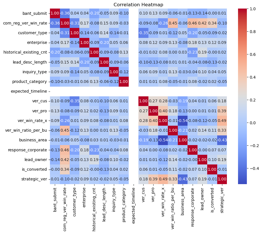
모델 실험

모델 성능 함수 정의

### 모델 성능 보기

def get_clf_eval(y_test, y_pred=None):
    confusion = confusion_matrix(y_test, y_pred, labels=[True, False])
    accuracy = accuracy_score(y_test, y_pred)
    precision = precision_score(y_test, y_pred, labels=[True, False])
    recall = recall_score(y_test, y_pred)
    F1 = f1_score(y_test, y_pred, labels=[True, False])

    print("오차행렬:\n", confusion)
    print("\n정확도: {:.4f}".format(accuracy))
    print("정밀도: {:.4f}".format(precision))
    print("재현율: {:.4f}".format(recall))
    print("F1: {:.4f}".format(F1))

XGBoost

오차행렬:
[[ 507 480]
[ 198 10675]]

정확도: 0.9428
정밀도: 0.7191
재현율: 0.5137
F1: 0.5993

DecisionTree

오차행렬:
[[ 618 369]
[ 326 10547]]

정확도: 0.9414
정밀도: 0.6547
재현율: 0.6261
F1: 0.6401

PCA 후 DecisionTree

오차행렬:
[[ 556 431]
[ 409 10464]]

정확도: 0.9292
정밀도: 0.5762
재현율: 0.5633
F1: 0.5697

RFE 후 DecisionTree

오차행렬:
[[ 618 369]
[ 311 10562]]

정확도: 0.9427
정밀도: 0.6652
재현율: 0.6261
F1: 0.6451

RandomForest

오차행렬:
[[ 544 443]
[ 203 10670]]

정확도: 0.9455
정밀도: 0.7282
재현율: 0.5512
F1: 0.6275

Ensemble 1_Randomforest+Gradientboosting+XGBoost+LightBoost F1: 0.5885
Ensemble2_Randomforet + GradientBoost + LogisticRegression + Decisiontree F1: 0.5567

→ Decisiontree val_data의 sum값이 가장 높게 나와서 decisiontree 하이퍼 파라미터 조정하는 걸로 시도

최종 제출

Decision tree - max_features 조정

오차행렬:
[[ 618 369]
[ 313 10560]]

정확도: 0.9425
정밀도: 0.6638
재현율: 0.6261
F1: 0.6444

877

💡 깨달은 점

DecisionTree모델로 가장 높은 성능이 나왔어서, 데이터 전처리에 시간을 더 쏟았어야 된다고 생각함.
Ensemble 모델이 어디서나 늘 높은 성능을 보이는 것은 아님.
주어진 데이터에 대해 얼마나 이해하고 있는지가 적합한 모델을 설계하는 데에 도움이 된다는 것을 앎.

B2B 영업기회 창출 예측 모델 개발

🪢 전체 Link

🔎 상세 내용

칼럼 4. ID0.4 + IT0.6 = strategic_ver로 통합

새로운 컬럼 생성 및 계산

test 적용

칼럼 7. response_corporate 전처리

대륙별로 response_corporate 값을 매핑하는 딕셔너리 생성

df_train DataFrame에서 expected_timeline 열의 모든 값을 문자열로 변환

데이터프레임에 함수 적용

test 적용

데이터프레임에 함수 적용

칼럼 8. expected_timeline 전처리

expected timeline 문구 대체 시도

0-3:0, 3-6:1, 6-9:2, 9-12:3, 12이상:4

대체할 값들

비슷한 문구를 찾고 해당하는 값으로 대체하는 함수 정의

df_train DataFrame에서 expected_timeline 열의 모든 값을 문자열로 변환

expected_timeline 열의 모든 값을 변경

test 적용

expected_timeline 열의 모든 값을 변경

str 변수 인코딩

학습데이터셋, 평가 데이터셋 분류

상관계수 파악

데이터프레임의 상관 행렬 계산

히트맵 그리기

모델 성능 함수 정의

최종 제출

💡 깨달은 점